GML ozonesonde and UFS-AQM
GML ozonesondes can be fetched and loaded with MONETIO. For this example, we use a pre-prepared dataset of the 100-m data[1] and compare to runs of developmental versions of the UFS-AQM regional model.
This example works with the CLI. (melodies-monet run).
Control file.
control_ufsaqm_ozonesonde.yaml
1# General Description:
2# Any key that is specific for a plot type will begin with ts for timeseries, ty for taylor
3# Opt: Specifying the variable or variable group is optional
4# For now all plots except time series average over the analysis window.
5# Setting axis values - If set_axis = True in data_proc section of each plot_grp the yaxis for the plot will be set based on the values specified in the obs section for each variable. If set_axis is set to False, then defaults will be used. 'vmin_plot' and 'vmax_plot' are needed for 'timeseries', 'spatial_overlay', and 'boxplot'. 'vdiff_plot' is needed for 'spatial_bias' plots and'ty_scale' is needed for 'taylor' plots. 'nlevels' or the number of levels used in the contour plot can also optionally be provided for spatial_overlay plot. If set_axis = True and the proper limits are not provided in the obs section, a warning will print, and the plot will be created using the default limits.
6analysis:
7 start_time: '2023-06-24-00:00:00' #UTC
8 end_time: '2023-06-25-00:00:00' #UTC
9 output_dir: ./output/ufsaqm_ozonesonde
10 debug: True
11
12model:
13 ufsaqm_cmaq52: # model label
14 files: 'example:ufsaqm:cmaq52_2023-06-24_20-21'
15 mod_type: 'ufs'
16 radius_of_influence: 19500 #meters: horizontal resolution * 1.5
17 mapping: #model species name : obs species name
18 gml-ozonesondes:
19 o3_ave: 'o3'
20 variables:
21 pres_pa_mid:
22 rename: pressure_model
23 unit_scale: 1
24 unit_scale_method: '*'
25 projection: ~
26 plot_kwargs: #Opt
27 color: 'red'
28 marker: '.'
29 linestyle: '-'
30
31 ufsaqm_cmaq54: # model label
32 files: 'example:ufsaqm:cmaq54_2023-06-24_20-21'
33 mod_type: 'ufs'
34 radius_of_influence: 19500 #meters: horizontal resolution * 1.5
35 mapping: #model species name : obs species name
36 gml-ozonesondes:
37 o3_ave: 'o3'
38 variables:
39 pres_pa_mid:
40 rename: pressure_model
41 unit_scale: 1
42 unit_scale_method: '*'
43 projection: ~
44 plot_kwargs: #Opt
45 color: 'cornflowerblue'
46 marker: '.'
47 linestyle: '-'
48
49obs:
50 gml-ozonesondes: # obs label
51 filename: 'example:gml-100m-ozonesondes:as-of-2024-02-09'
52 obs_type: sonde
53 variables: #Opt
54 o3:
55 unit_scale: 1000 #Opt Scaling factor (original ppmv, convert to ppbv)
56 unit_scale_method: '*' #Opt Multiply = '*' , Add = '+', subtract = '-', divide = '/'
57 nan_value: -1.0 # Opt Set this value to NaN
58 ylabel_plot: 'Ozone (ppbv)'
59 vmin_plot: 10.0 #Opt Min for y-axis during plotting. To apply to a plot, change restrict_yaxis = True.
60 vmax_plot: 100.0 #Opt Max for y-axis during plotting. To apply to a plot, change restrict_yaxis = True.
61 vdiff_plot: 20.0 #Opt +/- range to use in bias plots. To apply to a plot, change restrict_yaxis = True.
62 #nlevels_plot: 21 #Opt number of levels used in colorbar for contourf plot.
63 #regulatory: False #Opt compute regulatory functions
64 latitude:
65 unit_scale: 1
66 unit_scale_method: '*'
67 longitude:
68 unit_scale: 1
69 unit_scale_method: '*'
70 press:
71 rename: pressure_obs # name to convert this variable to
72 unit_scale: 100 # convert model hPa to Pa
73 unit_scale_method: '*'
74# temp:
75# rename: temperature_obs # name to convert this variable to
76# unit_scale: 0 # original in degree C
77# unit_scale_method: '-'
78
79plots:
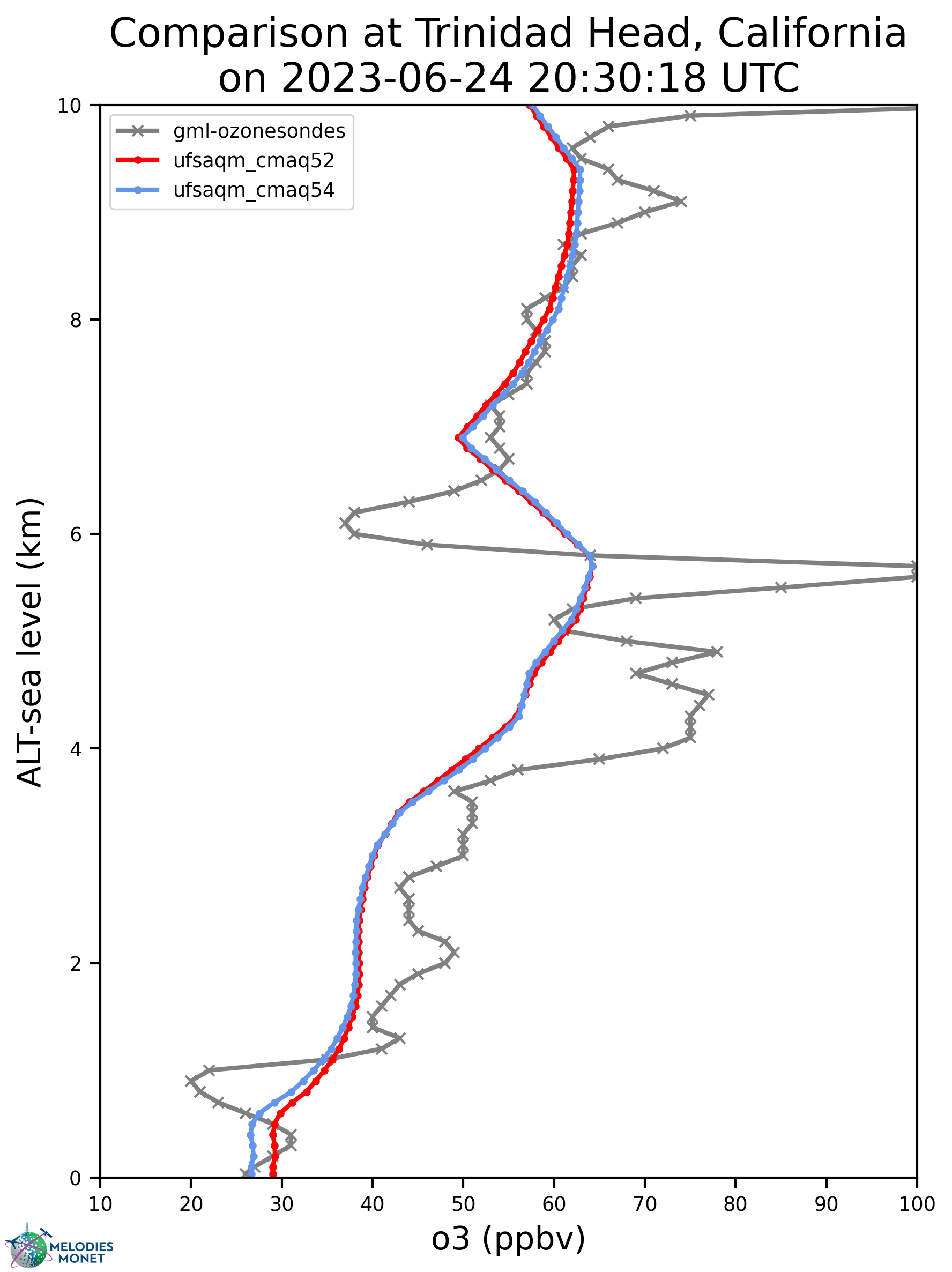
80 plot_grp1:
81 type: 'vertical_single_date' # plot type
82 fig_kwargs: #Opt to define figure options
83 figsize: [6,8] # figure size if multiple plots
84 default_plot_kwargs: # Opt to define defaults for all plots. Model kwargs overwrite these.
85 linewidth: 2.0
86 markersize: 5.
87 text_kwargs: #Opt
88 fontsize: 18.
89 domain_type: ['all'] #List of domain types: 'all' or any domain in obs file. (e.g., airnow: epa_region, state_name, siteid, etc.)
90 domain_name: ['CONUS'] #List of domain names. If domain_type = all domain_name is used in plot title.
91
92 altitude_range: [0,10]
93 altitude_method: ['sea level'] #choose from 'ground level' or 'sea level'
94 station_name: ['Trinidad Head, California']
95 compare_date_single: [2023,6,24,20,30,18]
96 monet_logo_position: [1] #1 is lower left, 4 is upper left.
97 data: ['gml-ozonesondes_ufsaqm_cmaq52', 'gml-ozonesondes_ufsaqm_cmaq54'] # make this a list of pairs in obs_model where the obs is the obs label and model is the model_label
98
99 data_proc:
100 #filter_dict: {'state_name':{'value':['CA','NY'],'oper':'isin'},'WS':{'value':1,'oper':'<'}}
101 #filter_string: state_name in ['CA','NY'] and WS < 1 # Uses pandas query method.
102 #rem_obs_by_nan_pct: {'group_var': 'siteid','pct_cutoff': 25,'times':'hourly'} # Groups by group_var, then removes all instances of groupvar where obs variable is > pct_cutoff % nan values
103 rem_obs_nan: True # True: Remove all points where model or obs variable is NaN. False: Remove only points where model variable is NaN.
104 #ts_select_time: 'time_local' #Time used for avg and plotting: Options: 'time' for UTC or 'time_local'
105 #ts_avg_window: 'H' # Options: None for no averaging or list pandas resample rule (e.g., 'H', 'D')
106 set_axis: True #If select True, add vmin_plot and vmax_plot for each variable in obs.
107
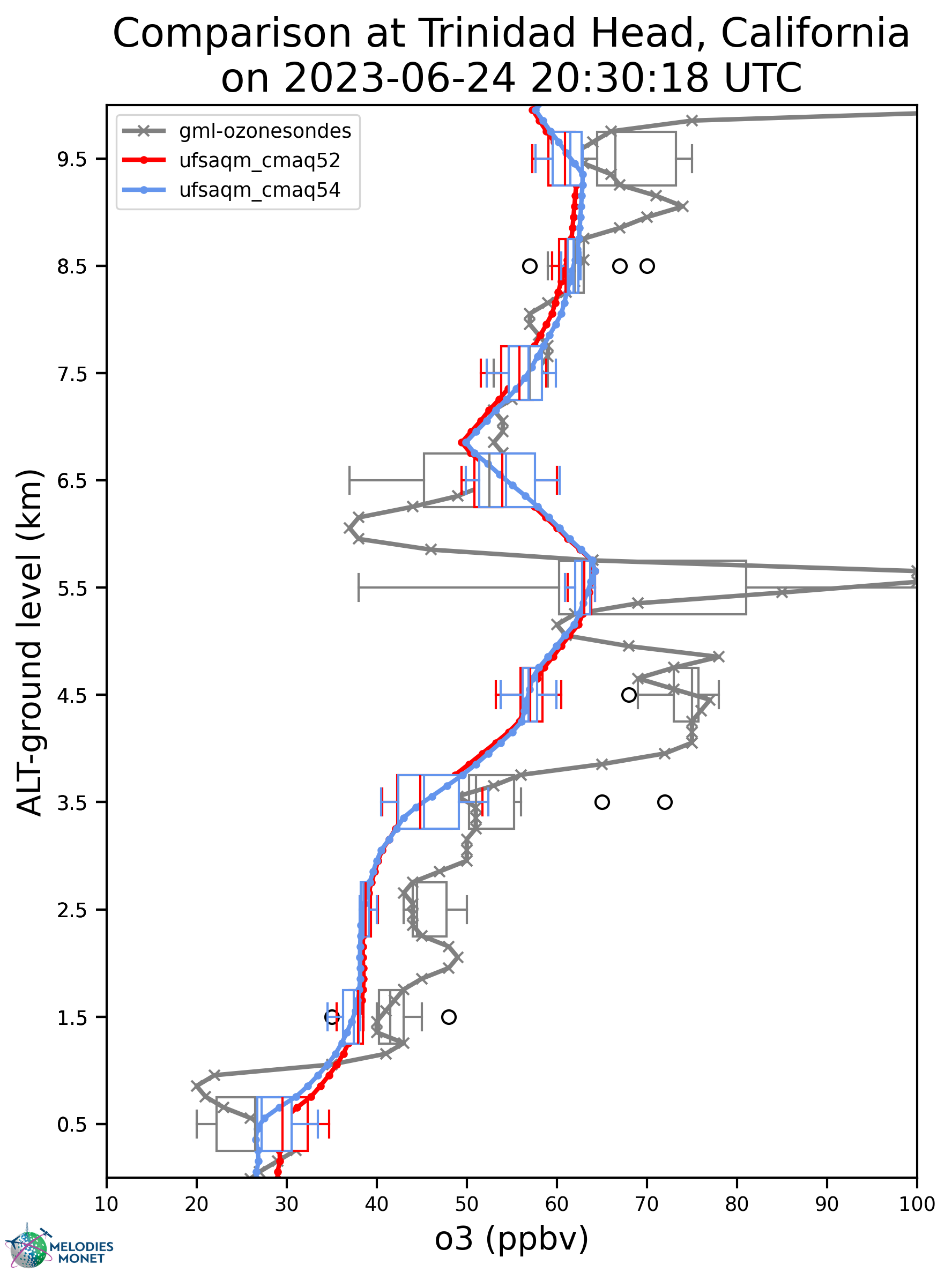
108 plot_grp2:
109 type: 'vertical_boxplot_os' # plot type
110 fig_kwargs: #Opt to define figure options
111 figsize: [6,8] # figure size if multiple plots
112 default_plot_kwargs: # Opt to define defaults for all plots. Model kwargs overwrite these.
113 linewidth: 2.0
114 markersize: 5.
115 text_kwargs: #Opt
116 fontsize: 18.
117 domain_type: ['all'] #List of domain types: 'all' or any domain in obs file. (e.g., airnow: epa_region, state_name, siteid, etc.)
118 domain_name: ['CONUS'] #List of domain names. If domain_type = all domain_name is used in plot title.
119
120 altitude_range: [0,10]
121 altitude_method: ['ground level'] #choose from 'ground level' or 'sea level'
122 station_name: ['Trinidad Head, California']
123 compare_date_single: [2023,6,24,20,30,18]
124 monet_logo_position: [1] #1 is lower left, 4 is upper left.
125 altitude_threshold_list: [0,1,2,3,4,5,6,7,8,9,10]
126 data: ['gml-ozonesondes_ufsaqm_cmaq52', 'gml-ozonesondes_ufsaqm_cmaq54'] # make this a list of pairs in obs_model where the obs is the obs label and model is the model_label
127
128 data_proc:
129 #filter_dict: {'state_name':{'value':['CA','NY'],'oper':'isin'},'WS':{'value':1,'oper':'<'}}
130 #filter_string: state_name in ['CA','NY'] and WS < 1 # Uses pandas query method.
131 #rem_obs_by_nan_pct: {'group_var': 'siteid','pct_cutoff': 25,'times':'hourly'} # Groups by group_var, then removes all instances of groupvar where obs variable is > pct_cutoff % nan values
132 rem_obs_nan: True # True: Remove all points where model or obs variable is NaN. False: Remove only points where model variable is NaN.
133 #ts_select_time: 'time_local' #Time used for avg and plotting: Options: 'time' for UTC or 'time_local'
134 #ts_avg_window: 'H' # Options: None for no averaging or list pandas resample rule (e.g., 'H', 'D')
135 set_axis: True #If select True, add vmin_plot and vmax_plot for each variable in obs.
136
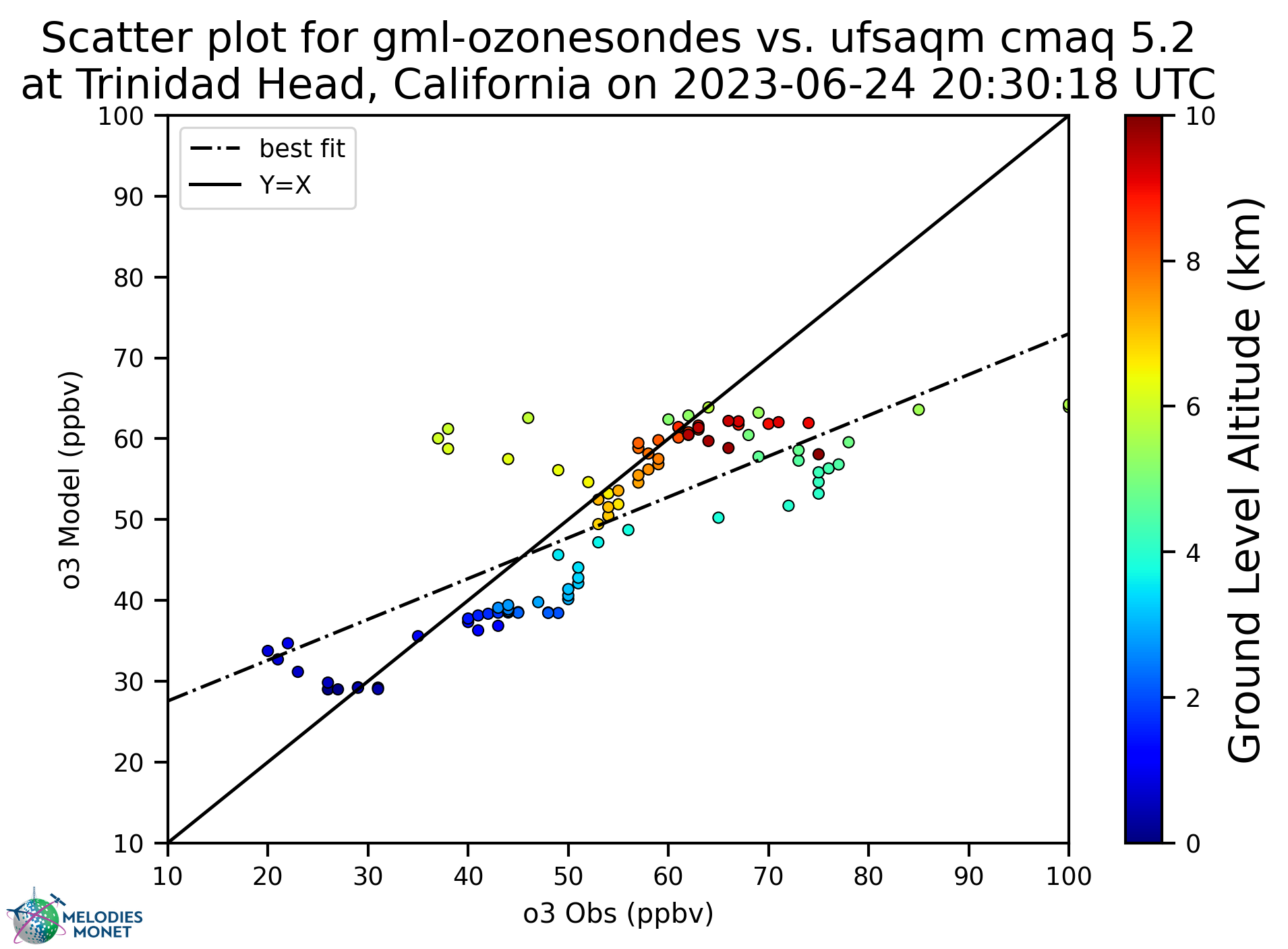
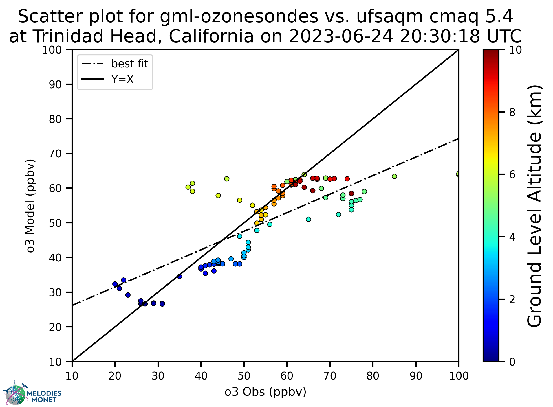
137 plot_grp3:
138 type: 'density_scatter_plot_os' # plot type
139 fig_kwargs: #Opt to define figure options
140 figsize: [10,8] # figure size if multiple plots
141 default_plot_kwargs: # Opt to define defaults for all plots. Model kwargs overwrite these.
142 linewidth: 2.0
143 markersize: 5.
144 text_kwargs: #Opt
145 fontsize: 18.
146 domain_type: ['all'] #List of domain types: 'all' or any domain in obs file. (e.g., airnow: epa_region, state_name, siteid, etc.)
147 domain_name: ['CONUS'] #List of domain names. If domain_type = all domain_name is used in plot title.
148
149 model_name_list: ['gml-ozonesondes', 'ufsaqm cmaq 5.2', 'ufsaqm cmaq 5.4']
150 altitude_range: [0,10]
151 altitude_method: ['ground level'] #choose from 'ground level' or 'sea level'
152
153# station_name: ['Boulder, Colorado']
154# compare_date_single: [2023,6,7,16,40,50]
155# compare_date_single: [2023,6,15,16,6,29]
156# compare_date_single: [2023,6,21,16,8,1]
157# compare_date_single: [2023,6,28,18,23,44]
158# compare_date_single: [2023,7,13,15,21,03]
159# compare_date_single: [2023,7,17,16,17,04]
160# compare_date_single: [2023,7,24,16,04,18]
161# compare_date_single: [2023,8,1,15,23,46]
162# compare_date_single: [2023,8,9,16,3,55]
163# compare_date_single: [2023,8,16,13,59,47]
164# compare_date_single: [2023,8,23,16,14,12]
165# compare_date_single: [2023,8,29,16,25,12]
166
167 station_name: ['Trinidad Head, California']
168# compare_date_single: [2023,6,12,1,2,7]
169# compare_date_single: [2023,6,14,23,5,6]
170 compare_date_single: [2023,6,24,20,30,18]
171# compare_date_single: [2023,7,03,20,38,41]
172# compare_date_single: [2023,7,22,21,43,40]
173# compare_date_single: [2023,8,4,22,16,11]
174# compare_date_single: [2023,8,10,20,25,51]
175# compare_date_single: [2023,8,18,20,9,52]
176 cmap_method: ['turbo']
177 monet_logo_position: [1] #1 is lower left, 4 is upper left.
178
179 data: ['gml-ozonesondes_ufsaqm_cmaq52', 'gml-ozonesondes_ufsaqm_cmaq54'] # make this a list of pairs in obs_model where the obs is the obs label and model is the model_label
180
181 data_proc:
182 #filter_dict: {'state_name':{'value':['CA','NY'],'oper':'isin'},'WS':{'value':1,'oper':'<'}}
183 #filter_string: state_name in ['CA','NY'] and WS < 1 # Uses pandas query method.
184 #rem_obs_by_nan_pct: {'group_var': 'siteid','pct_cutoff': 25,'times':'hourly'} # Groups by group_var, then removes all instances of groupvar where obs variable is > pct_cutoff % nan values
185 rem_obs_nan: True # True: Remove all points where model or obs variable is NaN. False: Remove only points where model variable is NaN.
186 #ts_select_time: 'time_local' #Time used for avg and plotting: Options: 'time' for UTC or 'time_local'
187 #ts_avg_window: 'H' # Options: None for no averaging or list pandas resample rule (e.g., 'H', 'D')
188 set_axis: True #If select True, add vmin_plot and vmax_plot for each variable in obs.
Plots