ISH and UFS-CHEM
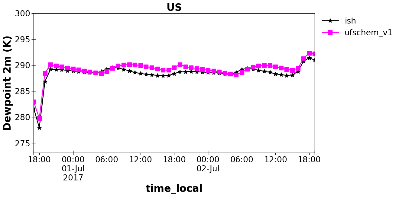
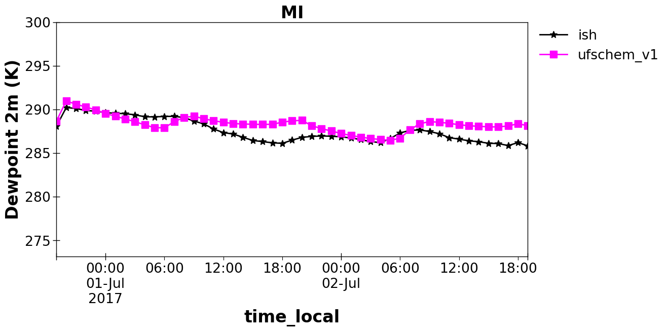
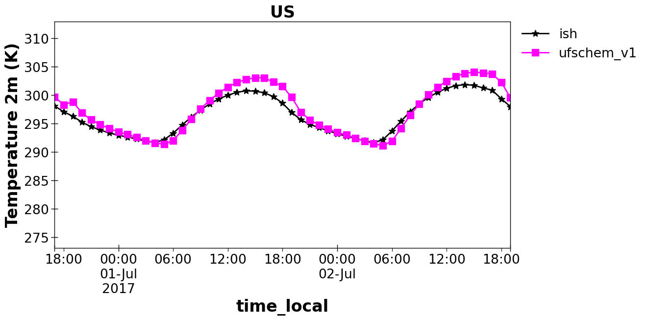
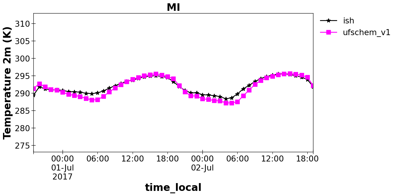
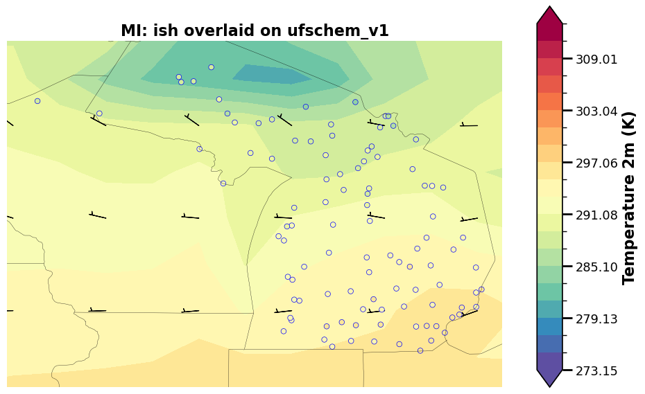
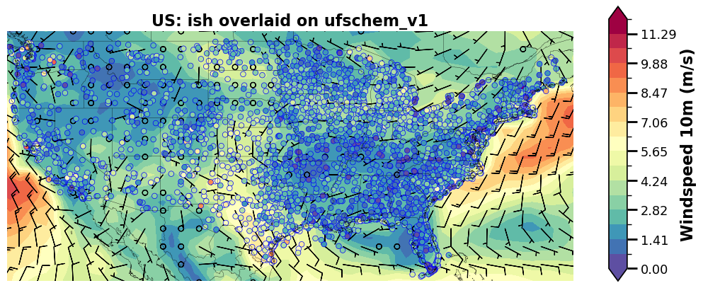
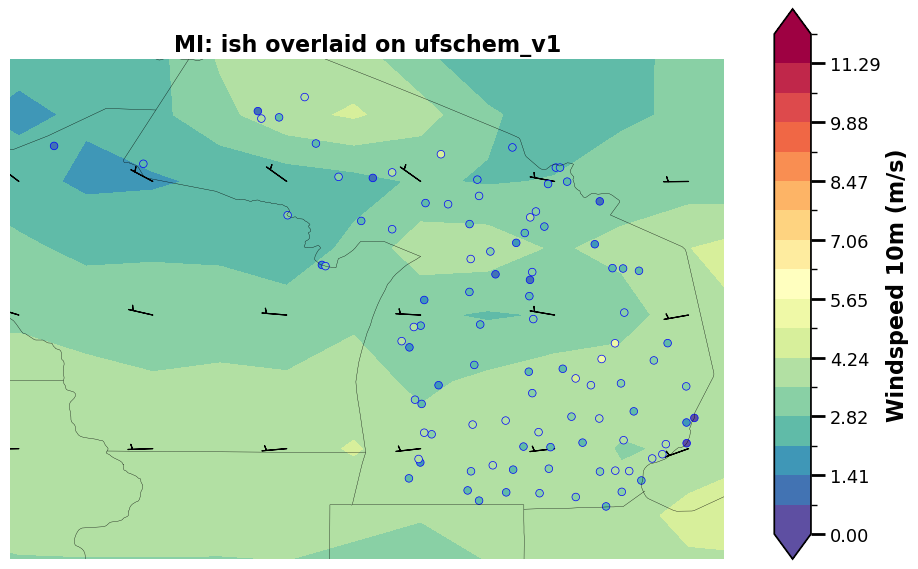
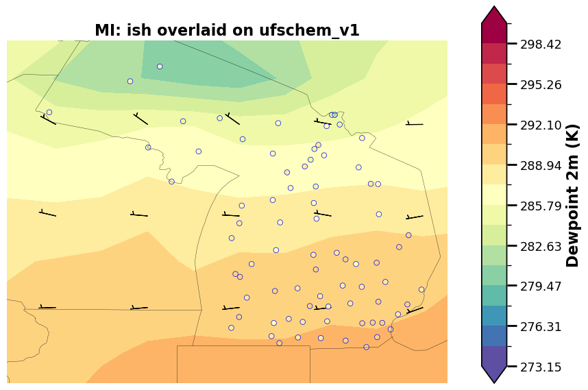
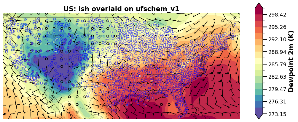
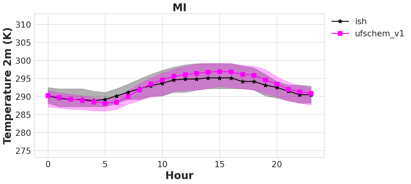
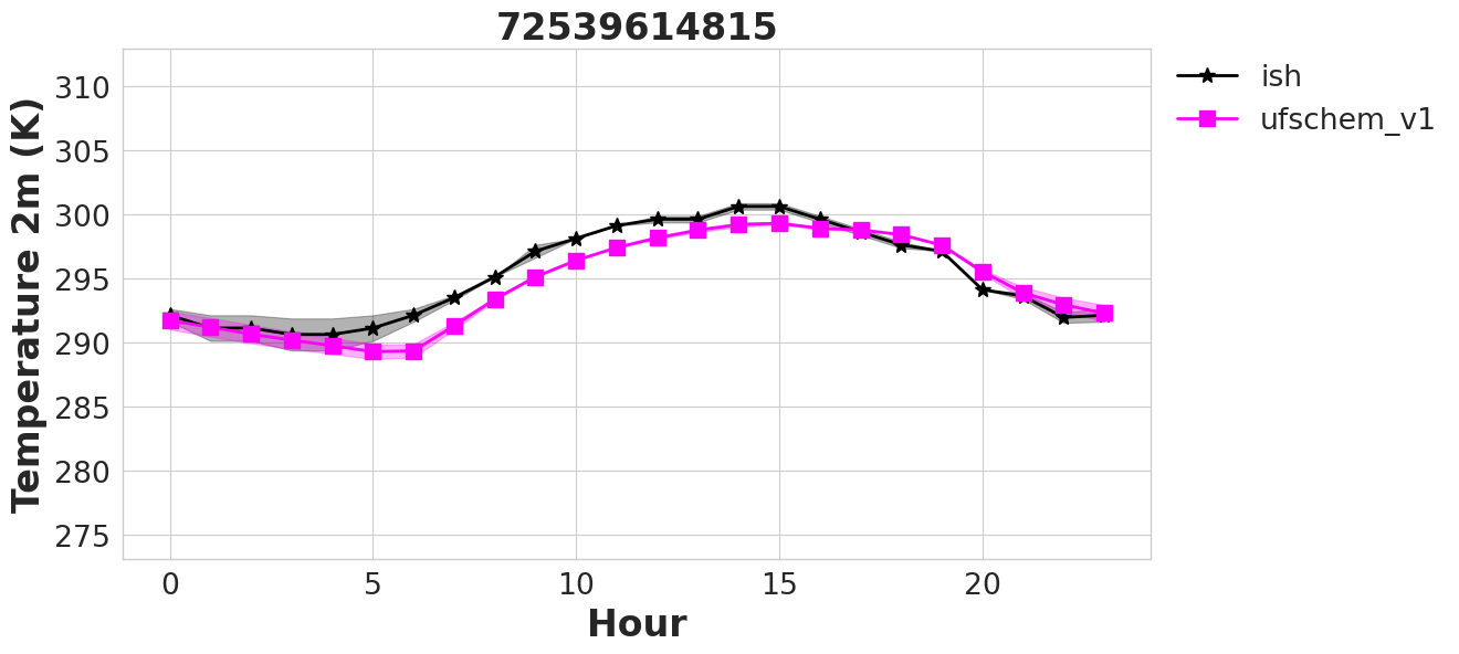
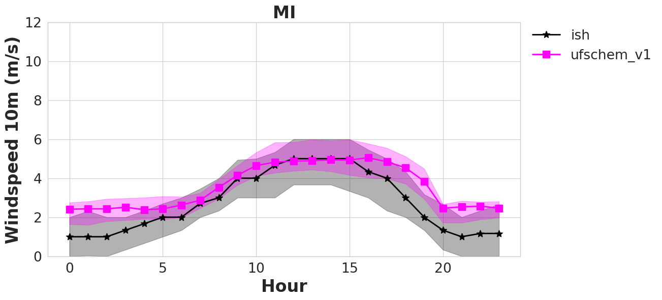
Our first example will demonstrate the basics available in MELODIES MONET to compare UFS-CHEM results against ISH surface observations for temperature, wind speed, and dewpoint.
ISH is a particularly useful for model evaluations because it is a global dataset. As you will see in the YAML file, we can create plots globally, for individual countries, and states. NOTE: MELODIES-MONET examples that use ISH will take longer to finish running due to the larger amount of data.
First, we import the melodies_monet.driver module.
from melodies_monet import driver
Analysis driver class
Now, lets create an instance of the analysis driver class, melodies_monet.driver.analysis.
It consists of these main parts:
model instances
observation instances
a paired instance of both
an = driver.analysis()
Initially, most of our analysis object’s attributes
are set to None, though some have meaningful defaults:
an
analysis(
    control='control.yaml',
    control_dict=None,
    models={},
    obs={},
    paired={},
    start_time=None,
    end_time=None,
    time_intervals=None,
    download_maps=True,
    output_dir=None,
    output_dir_save=None,
    output_dir_read=None,
    debug=False,
    save=None,
    read=None,
    regrid=False,
)
Control file
We set the YAML control file and begin by reading the file.
Note
Check out the Description of All YAML Options for info on how to create and modify these files.
an.control = "control_ish_ufschem-example.yaml"
an.read_control()
an.control_dict
Note: This is the complete file that was loaded.
  1# General Description:
  2# - Any key that is specific for a plot type will begin with `ts` for timeseries, `ty` for taylor.
  3# - Some keys/groups are optional.
  4# - For now, all plots except time series average over the analysis window.
  5# - Setting axis values
  6#   - If set_axis = True in data_proc section of each plot_grp,
  7#     the yaxis for the plot will be set based on the values
  8#     specified in the obs section for each variable.
  9#   - If set_axis is set to False, then defaults will be used.
 10#   - 'vmin_plot' and 'vmax_plot' are needed for
 11#     'timeseries', 'spatial_overlay', and 'boxplot'.
 12#   - 'vdiff_plot' is needed for 'spatial_bias' plots
 13#   - 'ty_scale' is needed for 'taylor' plots.
 14#   - 'nlevels' or the number of levels used in the contour plot can also optionally be provided for spatial_overlay plot.
 15#   - If set_axis = True and the proper limits are not provided in the obs section,
 16#     a warning will print, and the plot will be created using the default limits.
 17analysis:
 18  start_time: "2019-09-05-06:00:00" # UTC
 19  end_time: "2019-09-06-06:00:00" # UTC
 20  output_dir: ./output/airnow_wrfchem  # relative to the program using this control file
 21  #   Currently, the directory must exist or plot saving will error and fail.
 22  debug: True
 23
 24model:
 25  RACM_ESRL: # model label
 26    files: example:wrfchem:racm_esrl
 27    mod_type: "wrfchem"
 28    mod_kwargs:
 29      mech: "racm_esrl_vcp"
 30      surf_only_nc: True  # specify that we have only one vertical level; WRF-Chem specific
 31    radius_of_influence: 12000 # meters
 32    mapping: # of _model_ species name to _obs_ species name
 33      airnow: # specifically for the obs labeled 'airnow'
 34        PM2_5_DRY: "PM2.5"
 35        o3: "OZONE"
 36    projection: ~
 37    plot_kwargs: # optional
 38      color: "magenta"
 39      marker: "s"
 40      linestyle: "-"
 41  RACM_ESRL_VCP:
 42    files: example:wrfchem:racm_esrl_vcp
 43    mod_type: "wrfchem"
 44    mod_kwargs:
 45      mech: "racm_esrl_vcp"
 46      surf_only_nc: True
 47    radius_of_influence: 12000
 48    mapping:
 49      airnow:
 50        PM2_5_DRY: "PM2.5"
 51        o3: "OZONE"
 52    projection: ~
 53    plot_kwargs:
 54      color: "gold"
 55      marker: "o"
 56      linestyle: "-"
 57
 58obs:
 59  airnow: # obs label
 60    use_airnow: True
 61    filename: example:airnow:2019-09
 62    obs_type: pt_sfc
 63    variables: # optional
 64      OZONE:
 65        unit_scale: 1
 66        # ^ optional; Scaling factor
 67        unit_scale_method: "*"
 68        # ^ optional; Multiply = '*' , Add = '+', subtract = '-', divide = '/'
 69        nan_value: -1.0
 70        # ^ optional; When loading data, set this value to NaN
 71        ylabel_plot: "Ozone (ppbv)"
 72        # optional; set ylabel in order to include units and/or other info
 73        vmin_plot: 15.0
 74        # ^ optional; Min for y-axis during plotting.
 75        #   To apply to a plot, change restrict_yaxis = True.
 76        vmax_plot: 55.0
 77        # ^ optional; Max for y-axis during plotting.
 78        #   To apply to a plot, change restrict_yaxis = True.
 79        vdiff_plot: 20.0
 80        # ^ optional; +/- range to use in bias plots.
 81        #   To apply to a plot, change restrict_yaxis = True.
 82        nlevels_plot: 21
 83        # ^ optional; number of levels used in colorbar for contourf plot.
 84      PM2.5:
 85        unit_scale: 1
 86        unit_scale_method: "*"
 87        # obs_min: 0
 88        # ^ optional; set all values less than this value to NaN
 89        # obs_max: 100
 90        # ^ optional; set all values greater than this value to NaN
 91        nan_value: -1.0
 92        # Note: The obs_min, obs_max, and nan_values are set to NaN first
 93        # and then the unit conversion is applied.
 94        ylabel_plot: "PM2.5 (ug/m3)"
 95        ty_scale: 2.0 # optional; `ty_` indicates for Taylor diagram plot
 96        vmin_plot: 0.0
 97        vmax_plot: 22.0
 98        vdiff_plot: 15.0
 99        nlevels_plot: 23
100
101plots:
102  plot_grp1:
103    type: "timeseries" # plot type
104    fig_kwargs: # optional; to define figure options
105      figsize: [12, 6] # figure size (width, height) in inches
106    default_plot_kwargs:
107      # ^ optional; Define defaults for all plots.
108      #   Important: Model kwargs overwrite these.
109      linewidth: 2.0
110      markersize: 10.
111    text_kwargs: # optional
112      fontsize: 24.
113    domain_type: ["all", "state_name", "epa_region"]
114    # ^ List of domain types: 'all' or any domain in obs file.
115    #   (e.g., airnow: epa_region, state_name, siteid, etc.)
116    domain_name: ["CONUS", "CA", "R9"]
117    # ^ List of domain names. If domain_type = all,
118    #   the domain name is used in the plot title.
119    data: ["airnow_RACM_ESRL", "airnow_RACM_ESRL_VCP"]
120    # ^ make this a list of pairs in obs_model
121    #   where the obs is the obs label and model is the model_label
122    data_proc: # optional??
123      rem_obs_nan: True
124      # ^ True: Remove all points where model or obs variable is NaN.
125      #   False: Remove only points where model variable is NaN.
126      ts_select_time: "time_local"  # `ts_` indicates this is time series plot-specific
127      # ^ Time used for avg and plotting
128      #   Options: 'time' for UTC or 'time_local'
129      ts_avg_window: "h"
130      # ^ Options: None for no averaging, pandas resample rule (e.g., 'h', 'D')
131      set_axis: True
132      # ^ If true, add `vmin_plot` and `vmax_plot` for each variable in obs.
133
134  plot_grp2:
135    type: "taylor"
136    fig_kwargs:
137      figsize: [8, 8]
138    default_plot_kwargs:
139      linewidth: 2.0
140      markersize: 10.
141    text_kwargs:
142      fontsize: 16.
143    domain_type: ["all"]
144    domain_name: ["CONUS"]
145    data: ["airnow_RACM_ESRL", "airnow_RACM_ESRL_VCP"]
146    data_proc:
147      rem_obs_nan: True
148      set_axis: True
149
150  plot_grp3:
151    type: "spatial_bias"
152    fig_kwargs: # optional; For all spatial plots, specify map_kwargs here too.
153      states: True  # such as whether to show the state boundaries
154      figsize: [10, 5]
155    text_kwargs:
156      fontsize: 16.
157    domain_type: ["all",]
158    domain_name: ["CONUS"]
159    data: ["airnow_RACM_ESRL", "airnow_RACM_ESRL_VCP"]
160    data_proc:
161      rem_obs_nan: True
162      set_axis: True
163
164  plot_grp4:
165    type: "spatial_overlay"
166    fig_kwargs:
167      states: True
168      figsize: [10, 5]
169    text_kwargs:
170      fontsize: 16.
171    domain_type: ["all", "epa_region"]
172    domain_name: ["CONUS", "R9"]
173    data: ["airnow_RACM_ESRL", "airnow_RACM_ESRL_VCP"]
174    data_proc:
175      rem_obs_nan: True
176      set_axis: True
177
178  plot_grp5:
179    type: "boxplot"
180    fig_kwargs:
181      figsize: [8, 6]
182    text_kwargs:
183      fontsize: 20.
184    domain_type: ["all"]
185    domain_name: ["CONUS"]
186    data: ["airnow_RACM_ESRL", "airnow_RACM_ESRL_VCP"]
187    data_proc:
188      rem_obs_nan: True
189      set_axis: False
190
191  plot_grp6:
192    type: "scorecard"
193    fig_kwargs:
194      figsize: [15, 10]
195    text_kwargs:
196      fontsize: 20.
197    domain_type: ["all"]
198    domain_name: ["CONUS"]
199    region_name: ['epa_region']
200    region_list: ['R1','R2','R3','R4','R5','R6','R7','R8','R9','R10']
201    urban_rural_name: ['msa_name']
202    urban_rural_differentiate_value: ''
203    better_or_worse_method: 'NME'    #support 'RMSE', 'IOA' ,' NMB', 'NME'
204    model_name_list: ['AirNow','RACM_ESRL','RACM_ESRL_VCP']
205    data: ["airnow_RACM_ESRL", "airnow_RACM_ESRL_VCP"]
206    data_proc:
207      rem_obs_nan: True
208      set_axis: False
209
210  plot_grp7:
211    type: "multi_boxplot"
212    fig_kwargs:
213      figsize: [10, 8]
214    text_kwargs:
215      fontsize: 20.
216    domain_type: ["all"]
217    domain_name: ["CONUS"]
218    region_name: ['epa_region']
219    region_list: ['R1','R2','R3','R4','R5','R6','R7','R8','R9','R10']
220    model_name_list: ['AirNow','RACM_ESRL','RACM_ESRL_VCP']
221    data: ["airnow_RACM_ESRL", "airnow_RACM_ESRL_VCP"]
222    data_proc:
223      rem_obs_nan: True
224      set_axis: False
225
226  plot_grp8:
227    type: "csi"
228    fig_kwargs:
229      figsize: [10, 8]
230    text_kwargs:
231      fontsize: 20.
232    domain_type: ["all",'epa_region']
233    domain_name: ["CONUS",'R1']
234    threshold_list: [10,20,30,40,50,60,70,80,90,100]
235    score_name: 'Critical Success Index'  #can be used 'Critical Success Index' 'False Alarm Rate' 'Hit Rate'
236    model_name_list: ['RACM_ESRL','RACM_ESRL_VCP']
237    data: ["airnow_RACM_ESRL", "airnow_RACM_ESRL_VCP"]
238    data_proc:
239      rem_obs_nan: True
240      set_axis: False
241
242stats:
243  # Stats require positive numbers, so if you want to calculate temperature use Kelvin!
244  # Wind direction has special calculations for AirNow if obs name is 'WD'
245  stat_list: ["MB", "MdnB", "R2", "RMSE"]
246  # ^ List stats to calculate. Dictionary of definitions included
247  #   in submodule `plots/proc_stats`. Only stats listed below are currently working.
248  #   Full calc list:
249  #   ['STDO', 'STDP', 'MdnNB','MdnNE','NMdnGE',
250  #    'NO', 'NOP', 'NP', 'MO', 'MP', 'MdnO', 'MdnP',
251  #    'RM', 'RMdn', 'MB', 'MdnB', 'NMB', 'NMdnB', 'FB',
252  #    'ME','MdnE','NME', 'NMdnE', 'FE', 'R2', 'RMSE','d1',
253  #    'E1', 'IOA', 'AC']
254  round_output: 2 # optional; defaults to rounding to 3rd decimal place
255  output_table: False
256  # ^ Always outputs a .txt file.
257  #   Optional to also output a Matplotlib figure table (image).
258  output_table_kwargs: # optional
259    figsize: [7, 3]
260    fontsize: 12.
261    xscale: 1.4
262    yscale: 1.4
263    edges: "horizontal"
264  domain_type: ["all"]
265  domain_name: ["CONUS"]
266  data: ["airnow_RACM_ESRL", "airnow_RACM_ESRL_VCP"]
Now, some of our analysis object’s attributes are populated:
an
analysis(
    control='control_ish_ufschem-example.yaml',
    control_dict=...,
    models={},
    obs={},
    paired={},
    start_time=Timestamp('2017-07-01 00:00:00'),
    end_time=Timestamp('2017-07-03 00:00:00'),
    time_intervals=None,
    download_maps=True,
    output_dir='./output/ish_ufschem',
    output_dir_save='./output/ish_ufschem',
    output_dir_read='./output/ish_ufschem',
    debug=True,
    save=None,
    read=None,
    regrid=False,
)
Load the model data
The driver will automatically loop through the “models” found in the model section
of the YAML file and create an instance of melodies_monet.driver.model for each
that includes the
label
mapping information
file names (can be expressed using a glob expression)
xarray object
Note: Relevant control file section.
 1model:
 2  RACM_ESRL: # model label
 3    files: example:wrfchem:racm_esrl
 4    mod_type: "wrfchem"
 5    mod_kwargs:
 6      mech: "racm_esrl_vcp"
 7      surf_only_nc: True  # specify that we have only one vertical level; WRF-Chem specific
 8    radius_of_influence: 12000 # meters
 9    mapping: # of _model_ species name to _obs_ species name
10      airnow: # specifically for the obs labeled 'airnow'
11        PM2_5_DRY: "PM2.5"
12        o3: "OZONE"
13    projection: ~
14    plot_kwargs: # optional
15      color: "magenta"
16      marker: "s"
17      linestyle: "-"
18  RACM_ESRL_VCP:
19    files: example:wrfchem:racm_esrl_vcp
20    mod_type: "wrfchem"
21    mod_kwargs:
22      mech: "racm_esrl_vcp"
23      surf_only_nc: True
24    radius_of_influence: 12000
25    mapping:
26      airnow:
27        PM2_5_DRY: "PM2.5"
28        o3: "OZONE"
29    projection: ~
30    plot_kwargs:
31      color: "gold"
32      marker: "o"
33      linestyle: "-"
an.open_models()
ufs
example:ufschem:2017-07
**** Reading UFS-AQM or UFS-Chem model output...
Performing extra model calculations...
Calculating modeled Dewpoint...
Calculating modeled relative humidity...
Calculating modeled windspeed...
Calculating modeled wind direction...
Applying open_models()
populates the models attribute.
an.models
{'ufschem_v1': model(
     model='ufs',
     is_global=True,
     radius_of_influence=100000,
     mod_kwargs={'surf_only': True, 'sfc_varlist': ['tmp2m', 'spfh2m', 'ugrd10m', 'vgrd10m'], 'fname_sfc': ['/home/rschwantes/.cache/pooch/5207e0e702072b5e37fd507da111f78d-2017_07_01_03_ufschemv1_sfc.nc'], 'var_list': ['lat', 'lon', 'phalf', 'tmp', 'pressfc', 'dpres', 'hgtsfc', 'delz']},
     file_str='example:ufschem:2017-07',
     label='ufschem_v1',
     obj=...,
     extra_calc={'dewpoint': {'pres_calc': 'surfpres_pa', 'specific_hum': 'spfh2m'}, 'rel_hum': {'pres_calc': 'surfpres_pa', 'specific_hum': 'spfh2m', 'temp_calc': 'tmp2m'}, 'windspeed': {'u_comp': 'ugrd10m', 'v_comp': 'vgrd10m'}, 'winddir': {'u_comp': 'ugrd10m', 'v_comp': 'vgrd10m'}, 'wind_barb': {'u_comp': 'ugrd10m', 'v_comp': 'vgrd10m'}, 'rose_plot': {'model_wdir': 'winddir', 'model_wspd': 'windspeed'}},
     mapping={'ish': {'tmp2m': 't', 'windspeed': 'ws', 'dewpoint': 'dpt'}},
     variable_dict={'surfpres_pa': 'None', 'spfh2m': 'None', 'tmp2m': 'None', 'ugrd10m': 'None', 'vgrd10m': 'None', 'winddir': 'None', 'windspeed': 'None'},
     label='ufschem_v1',
     ...
 )}
We can access the underlying dataset with the
obj attribute.
an.models['ufschem_v1'].obj
<xarray.Dataset> Size: 320MB
Dimensions:        (y: 192, x: 384, time: 72, z: 1)
Coordinates:
    latitude       (y, x) float64 590kB dask.array<chunksize=(192, 384), meta=np.ndarray>
    longitude      (y, x) float64 590kB dask.array<chunksize=(192, 384), meta=np.ndarray>
  * time           (time) datetime64[ns] 576B 2017-07-01T01:00:00 ... 2017-07-04
  * x              (x) float64 3kB 0.0 0.9375 1.875 2.812 ... 357.2 358.1 359.1
  * y              (y) float64 2kB 89.28 88.36 87.42 ... -87.42 -88.36 -89.28
Dimensions without coordinates: z
Data variables: (12/14)
    temperature_k  (time, z, y, x) float32 21MB dask.array<chunksize=(1, 1, 192, 384), meta=np.ndarray>
    surfpres_pa    (time, z, y, x) float32 21MB dask.array<chunksize=(1, 1, 192, 384), meta=np.ndarray>
    dp_pa          (time, z, y, x) float32 21MB dask.array<chunksize=(1, 1, 192, 384), meta=np.ndarray>
    surfalt_m      (time, z, y, x) float32 21MB dask.array<chunksize=(1, 1, 192, 384), meta=np.ndarray>
    dz_m           (time, z, y, x) float32 21MB dask.array<chunksize=(1, 1, 192, 384), meta=np.ndarray>
    pres_pa_mid    (time, z, y, x) float64 42MB dask.array<chunksize=(1, 1, 192, 384), meta=np.ndarray>
    ...             ...
    ugrd10m        (time, z, y, x) float32 21MB dask.array<chunksize=(1, 1, 192, 384), meta=np.ndarray>
    vgrd10m        (time, z, y, x) float32 21MB dask.array<chunksize=(1, 1, 192, 384), meta=np.ndarray>
    dewpoint       (time, z, y, x) float32 21MB dask.array<chunksize=(1, 1, 192, 384), meta=np.ndarray>
    rel_hum        (time, z, y, x) float32 21MB dask.array<chunksize=(1, 1, 192, 384), meta=np.ndarray>
    windspeed      (time, z, y, x) float32 21MB dask.array<chunksize=(1, 1, 192, 384), meta=np.ndarray>
    winddir        (time, z, y, x) float32 21MB 243.3 244.2 ... 352.7 351.9
Attributes:
    grid:         gaussian
    grid_id:      1
    hydrostatic:  non-hydrostatic
    im:           384
    jm:           192
    ncnsto:       139
    source:       FV3GFS
    NCO:          netCDF Operators version 5.0.7 (Homepage = http://nco.sf.ne...
    ak:           [0. 0.]
    bk:           [0.99467119 1.        ]
history: Fri Feb 27 09:53:22 2026: ncrcat 20170701_dynf001.nc 201707...Load the observational data
As with the model data, the driver will loop through the “observations” found in
the obs section of the YAML file and create an instance of
melodies_monet.driver.observation for each.
Note: Relevant control file section.
 1obs:
 2  airnow: # obs label
 3    use_airnow: True
 4    filename: example:airnow:2019-09
 5    obs_type: pt_sfc
 6    variables: # optional
 7      OZONE:
 8        unit_scale: 1
 9        # ^ optional; Scaling factor
10        unit_scale_method: "*"
11        # ^ optional; Multiply = '*' , Add = '+', subtract = '-', divide = '/'
12        nan_value: -1.0
13        # ^ optional; When loading data, set this value to NaN
14        ylabel_plot: "Ozone (ppbv)"
15        # optional; set ylabel in order to include units and/or other info
16        vmin_plot: 15.0
17        # ^ optional; Min for y-axis during plotting.
18        #   To apply to a plot, change restrict_yaxis = True.
19        vmax_plot: 55.0
20        # ^ optional; Max for y-axis during plotting.
21        #   To apply to a plot, change restrict_yaxis = True.
22        vdiff_plot: 20.0
23        # ^ optional; +/- range to use in bias plots.
24        #   To apply to a plot, change restrict_yaxis = True.
25        nlevels_plot: 21
26        # ^ optional; number of levels used in colorbar for contourf plot.
27      PM2.5:
28        unit_scale: 1
29        unit_scale_method: "*"
30        # obs_min: 0
31        # ^ optional; set all values less than this value to NaN
32        # obs_max: 100
33        # ^ optional; set all values greater than this value to NaN
34        nan_value: -1.0
35        # Note: The obs_min, obs_max, and nan_values are set to NaN first
36        # and then the unit conversion is applied.
37        ylabel_plot: "PM2.5 (ug/m3)"
38        ty_scale: 2.0 # optional; `ty_` indicates for Taylor diagram plot
39        vmin_plot: 0.0
40        vmax_plot: 22.0
41        vdiff_plot: 15.0
42        nlevels_plot: 23
an.open_obs()
Performing extra calculations for obs...
an.obs
{'ish': observation(
     obs='ish',
     label='ish',
     file='example:ish:2017-07',
     obj=...,
     extra_calc={'rose_plot': {'obs_wdir': 'wdir', 'obs_wspd': 'ws'}},
     type='pt_src',
     sat_type=None,
     sat_method=None,
     data_proc=None,
     variable_dict={'t': {'unit_scale': 273.15, 'unit_scale_method': '+', 'nan_value': -1.0, 'ylabel_plot': 'Temperature 2m (K)', 'xlabel_plot': 'Temperature 2m (K)', 'vmin_plot': 273.15, 'vmax_plot': 313, 'vdiff_plot': 20.0, 'nlevels_plot': 21}, 'ws': {'unit_scale': 1, 'unit_scale_method': '*', 'nan_value': -1.0, 'ylabel_plot': 'Windspeed 10m (m/s)', 'xlabel_plot': 'Windspeed 10m (m/s)', 'vmin_plot': 0, 'vmax_plot': 12, 'vdiff_plot': 4, 'nlevels_plot': 18}, 'wdir': {'unit_scale': 1, 'unit_scale_method': '*', 'nan_value': -1.0, 'ylabel_plot': 'Wind Direction 10m (deg)', 'xlabel_plot': 'Wind Direction 10m (deg)', 'vmin_plot': 0, 'vmax_plot': 370, 'vdiff_plot': 4, 'nlevels_plot': 18}, 'dpt': {'unit_scale': 273.15, 'unit_scale_method': '+', 'nan_value': -1.0, 'ylabel_plot': 'Dewpoint 2m (K)', 'xlabel_plot': 'Dewpoint 2m (K)', 'vmin_plot': 273.15, 'vmax_plot': 300, 'vdiff_plot': 4, 'nlevels_plot': 18}},
     resample=None,
     time_var=None,
     regrid_method=None,
 )}
an.obs['ish'].obj
<xarray.Dataset> Size: 48MB
Dimensions:       (time: 49, y: 1, x: 12321)
Coordinates:
  * time          (time) datetime64[ns] 392B 2017-07-01 ... 2017-07-03
    siteid        (x) <U11 542kB ...
    latitude      (x) float64 99kB ...
    longitude     (x) float64 99kB ...
  * x             (x) int64 99kB 0 1 2 3 4 5 ... 12316 12317 12318 12319 12320
Dimensions without coordinates: y
Data variables: (12/19)
    varlength     (time, y, x) float64 5MB ...
    wdir          (time, y, x) float64 5MB nan nan 320.0 80.0 ... nan nan nan
    ws            (time, y, x) float64 5MB nan nan 4.0 2.0 ... nan nan nan nan
    ceiling       (time, y, x) float64 5MB ...
    vsb           (time, y, x) float64 5MB ...
    t             (time, y, x) float64 5MB nan nan 271.1 275.1 ... nan nan nan
    ...            ...
    icao          (y, x) <U4 197kB ...
    elevation     (y, x) float64 99kB ...
    utcoffset     (y, x) float64 99kB ...
    begin         (y, x) datetime64[ns] 99kB ...
    end           (y, x) datetime64[ns] 99kB ...
time_local (time, y, x) datetime64[ns] 5MB ...Pair model and observational data
Now, we create a melodies_monet.driver.pair for each model–obs pair
using the pair_data() routine.
%%time

an.pair_data()
an.paired
{'ish_ufschem_v1': pair(
     type='pt_sfc',
     radius_of_influence=1000000.0,
     obs='ish',
     model='ufschem_v1',
     model_vars=['tmp2m', 'windspeed', 'dewpoint'],
     obs_vars=['t', 'ws', 'dpt'],
     filename='ish_ufschem_v1.nc',
 )}
an.paired['ish_ufschem_v1']
pair(
    type='pt_sfc',
    radius_of_influence=1000000.0,
    obs='ish',
    model='ufschem_v1',
    model_vars=['tmp2m', 'windspeed', 'dewpoint'],
    obs_vars=['t', 'ws', 'dpt'],
    filename='ish_ufschem_v1.nc',
)
MELODIES-MONET now contains several meteorological capabilities
In addition to previous capabilites and plots, users can now:
Specify wind barbs
Note: users may experience longer wait times if they wish to plot wind barbs
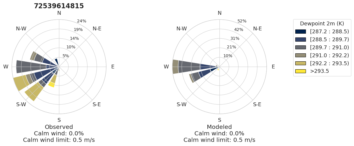
Create rose plots for pollution and wind speed
Rose plots can be aggregated at the Country-, EPA region-, and MSA-scale
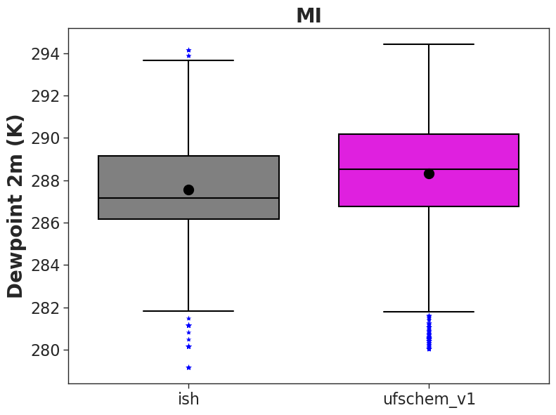
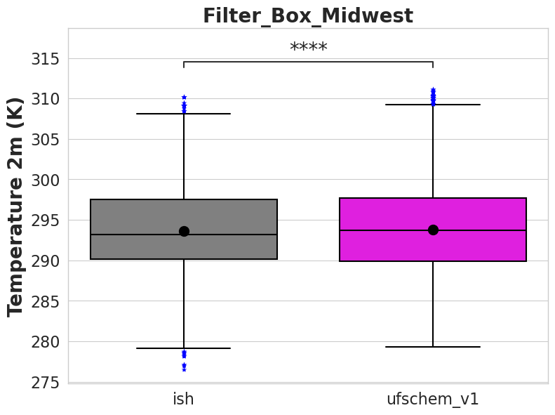
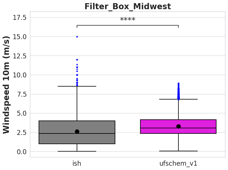
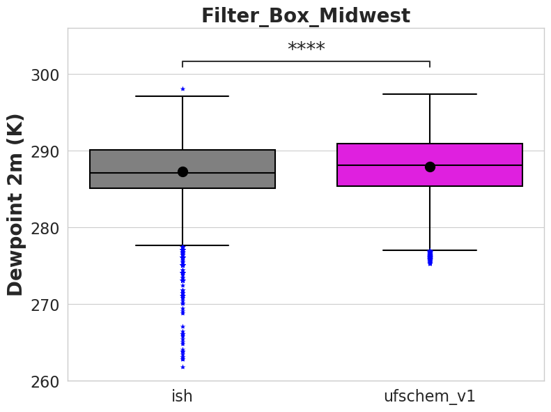
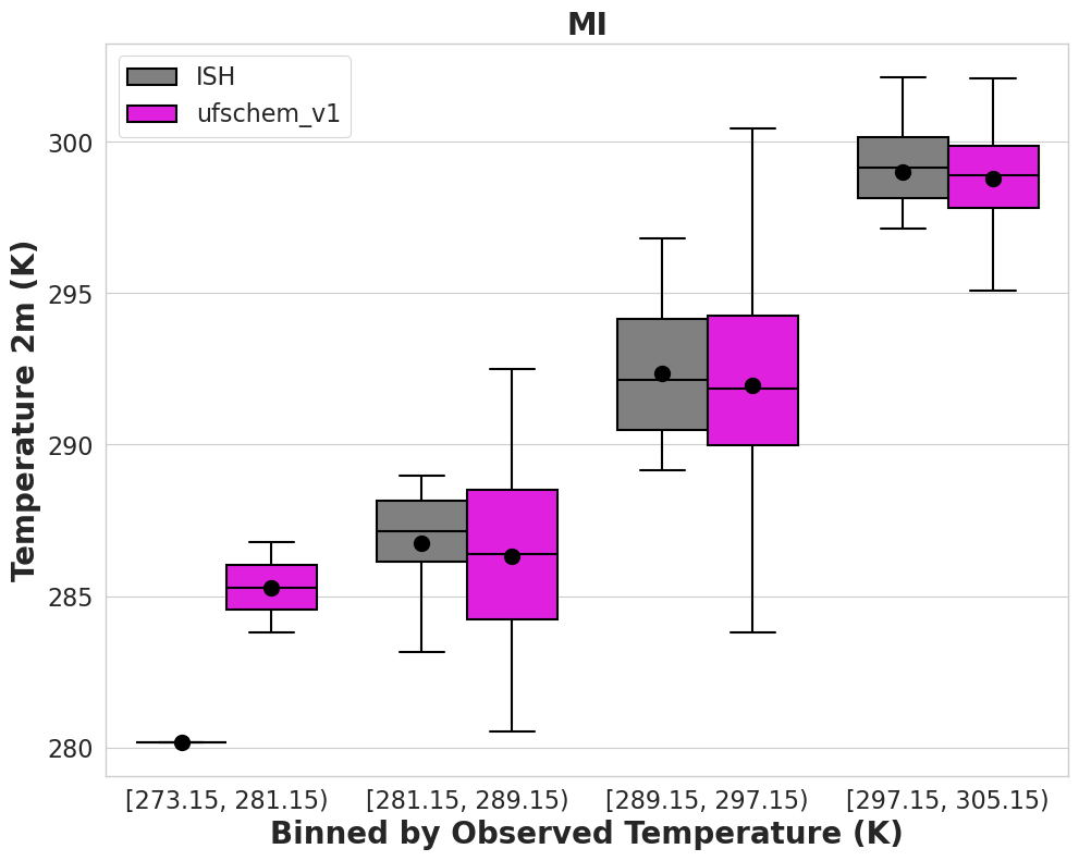
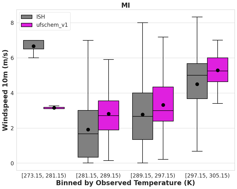
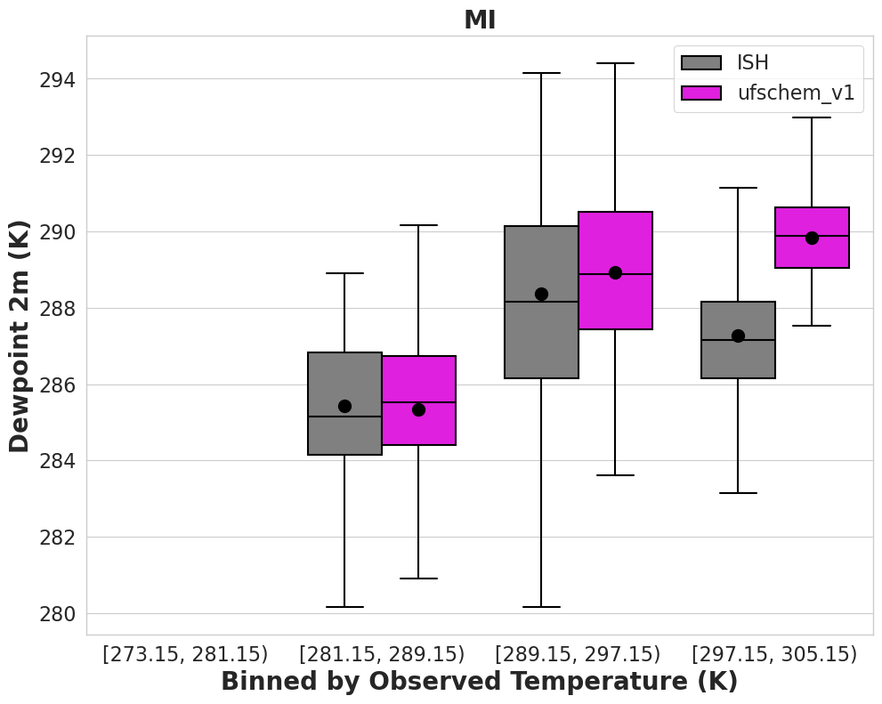
Create boxplots on given intervals for any of the supported meteorological variables
Mark statistical significance on boxplots
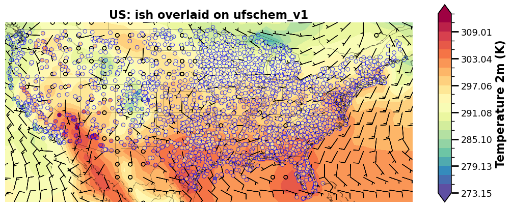
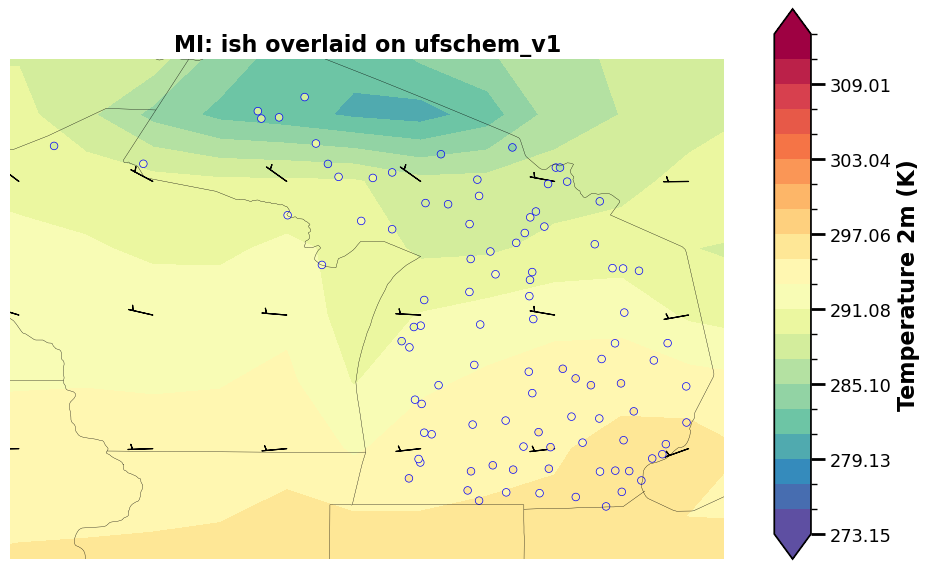
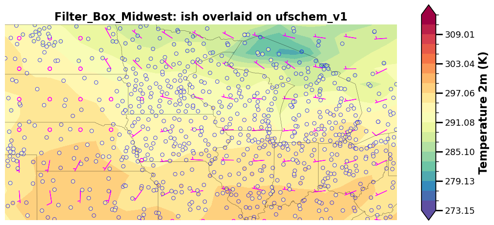
Plot
The plotting() routine produces plots.
Note: Relevant control file section.
  1plots:
  2  plot_grp1:
  3    type: "timeseries" # plot type
  4    fig_kwargs: # optional; to define figure options
  5      figsize: [12, 6] # figure size (width, height) in inches
  6    default_plot_kwargs:
  7      # ^ optional; Define defaults for all plots.
  8      #   Important: Model kwargs overwrite these.
  9      linewidth: 2.0
 10      markersize: 10.
 11    text_kwargs: # optional
 12      fontsize: 24.
 13    domain_type: ["all", "state_name", "epa_region"]
 14    # ^ List of domain types: 'all' or any domain in obs file.
 15    #   (e.g., airnow: epa_region, state_name, siteid, etc.)
 16    domain_name: ["CONUS", "CA", "R9"]
 17    # ^ List of domain names. If domain_type = all,
 18    #   the domain name is used in the plot title.
 19    data: ["airnow_RACM_ESRL", "airnow_RACM_ESRL_VCP"]
 20    # ^ make this a list of pairs in obs_model
 21    #   where the obs is the obs label and model is the model_label
 22    data_proc: # optional??
 23      rem_obs_nan: True
 24      # ^ True: Remove all points where model or obs variable is NaN.
 25      #   False: Remove only points where model variable is NaN.
 26      ts_select_time: "time_local"  # `ts_` indicates this is time series plot-specific
 27      # ^ Time used for avg and plotting
 28      #   Options: 'time' for UTC or 'time_local'
 29      ts_avg_window: "h"
 30      # ^ Options: None for no averaging, pandas resample rule (e.g., 'h', 'D')
 31      set_axis: True
 32      # ^ If true, add `vmin_plot` and `vmax_plot` for each variable in obs.
 33
 34  plot_grp2:
 35    type: "taylor"
 36    fig_kwargs:
 37      figsize: [8, 8]
 38    default_plot_kwargs:
 39      linewidth: 2.0
 40      markersize: 10.
 41    text_kwargs:
 42      fontsize: 16.
 43    domain_type: ["all"]
 44    domain_name: ["CONUS"]
 45    data: ["airnow_RACM_ESRL", "airnow_RACM_ESRL_VCP"]
 46    data_proc:
 47      rem_obs_nan: True
 48      set_axis: True
 49
 50  plot_grp3:
 51    type: "spatial_bias"
 52    fig_kwargs: # optional; For all spatial plots, specify map_kwargs here too.
 53      states: True  # such as whether to show the state boundaries
 54      figsize: [10, 5]
 55    text_kwargs:
 56      fontsize: 16.
 57    domain_type: ["all",]
 58    domain_name: ["CONUS"]
 59    data: ["airnow_RACM_ESRL", "airnow_RACM_ESRL_VCP"]
 60    data_proc:
 61      rem_obs_nan: True
 62      set_axis: True
 63
 64  plot_grp4:
 65    type: "spatial_overlay"
 66    fig_kwargs:
 67      states: True
 68      figsize: [10, 5]
 69    text_kwargs:
 70      fontsize: 16.
 71    domain_type: ["all", "epa_region"]
 72    domain_name: ["CONUS", "R9"]
 73    data: ["airnow_RACM_ESRL", "airnow_RACM_ESRL_VCP"]
 74    data_proc:
 75      rem_obs_nan: True
 76      set_axis: True
 77
 78  plot_grp5:
 79    type: "boxplot"
 80    fig_kwargs:
 81      figsize: [8, 6]
 82    text_kwargs:
 83      fontsize: 20.
 84    domain_type: ["all"]
 85    domain_name: ["CONUS"]
 86    data: ["airnow_RACM_ESRL", "airnow_RACM_ESRL_VCP"]
 87    data_proc:
 88      rem_obs_nan: True
 89      set_axis: False
 90
 91  plot_grp6:
 92    type: "scorecard"
 93    fig_kwargs:
 94      figsize: [15, 10]
 95    text_kwargs:
 96      fontsize: 20.
 97    domain_type: ["all"]
 98    domain_name: ["CONUS"]
 99    region_name: ['epa_region']
100    region_list: ['R1','R2','R3','R4','R5','R6','R7','R8','R9','R10']
101    urban_rural_name: ['msa_name']
102    urban_rural_differentiate_value: ''
103    better_or_worse_method: 'NME'    #support 'RMSE', 'IOA' ,' NMB', 'NME'
104    model_name_list: ['AirNow','RACM_ESRL','RACM_ESRL_VCP']
105    data: ["airnow_RACM_ESRL", "airnow_RACM_ESRL_VCP"]
106    data_proc:
107      rem_obs_nan: True
108      set_axis: False
109
110  plot_grp7:
111    type: "multi_boxplot"
112    fig_kwargs:
113      figsize: [10, 8]
114    text_kwargs:
115      fontsize: 20.
116    domain_type: ["all"]
117    domain_name: ["CONUS"]
118    region_name: ['epa_region']
119    region_list: ['R1','R2','R3','R4','R5','R6','R7','R8','R9','R10']
120    model_name_list: ['AirNow','RACM_ESRL','RACM_ESRL_VCP']
121    data: ["airnow_RACM_ESRL", "airnow_RACM_ESRL_VCP"]
122    data_proc:
123      rem_obs_nan: True
124      set_axis: False
125
126  plot_grp8:
127    type: "csi"
128    fig_kwargs:
129      figsize: [10, 8]
130    text_kwargs:
131      fontsize: 20.
132    domain_type: ["all",'epa_region']
133    domain_name: ["CONUS",'R1']
134    threshold_list: [10,20,30,40,50,60,70,80,90,100]
135    score_name: 'Critical Success Index'  #can be used 'Critical Success Index' 'False Alarm Rate' 'Hit Rate'
136    model_name_list: ['RACM_ESRL','RACM_ESRL_VCP']
137    data: ["airnow_RACM_ESRL", "airnow_RACM_ESRL_VCP"]
138    data_proc:
139      rem_obs_nan: True
140      set_axis: False
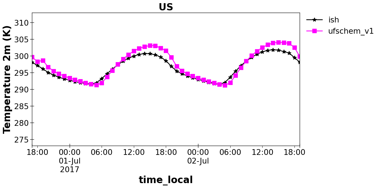
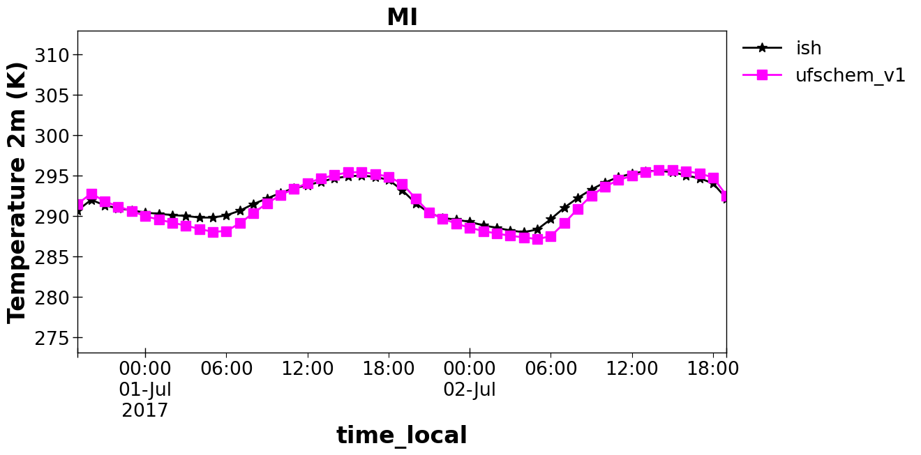
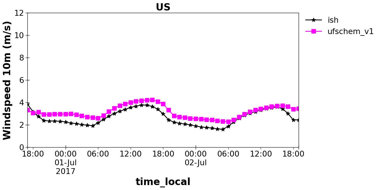
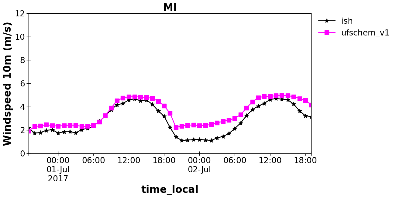
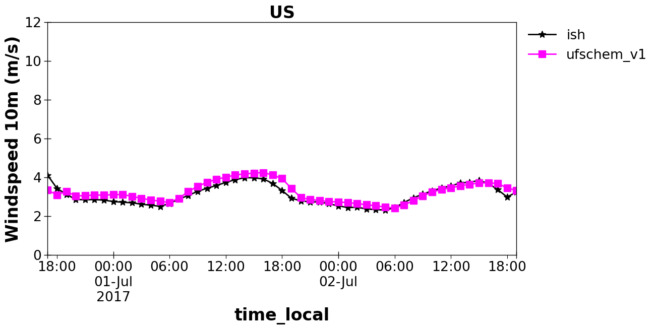
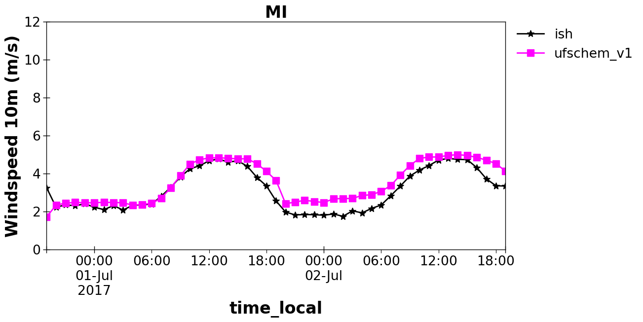
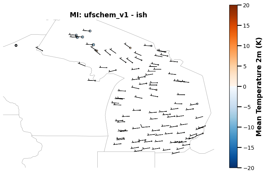
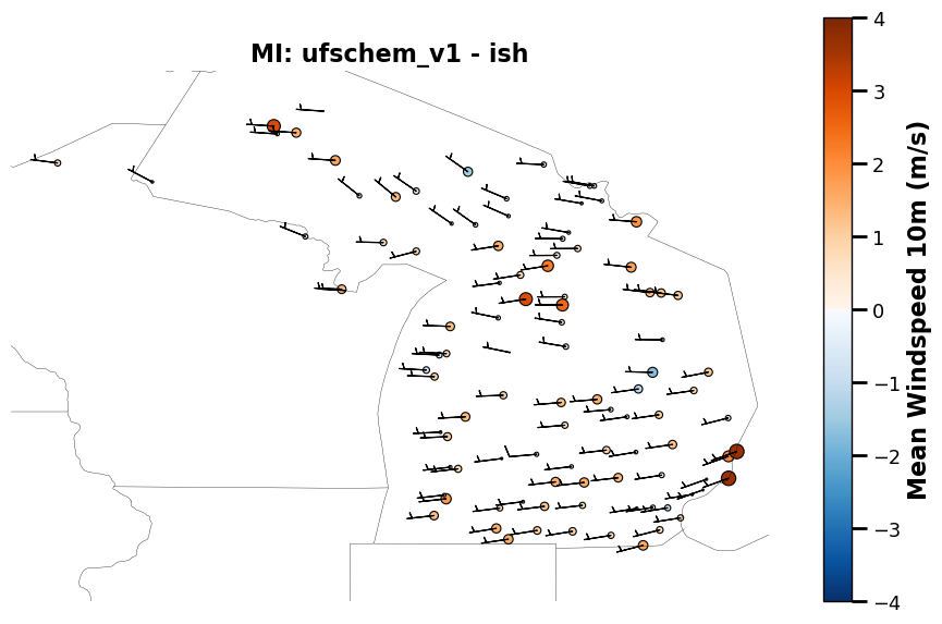
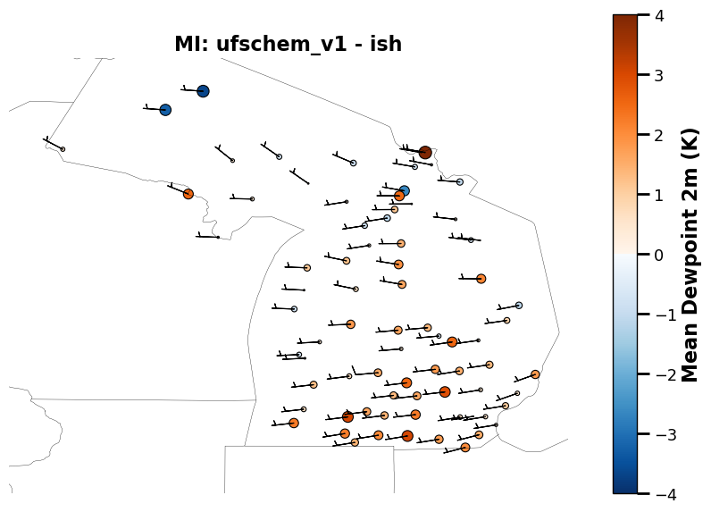
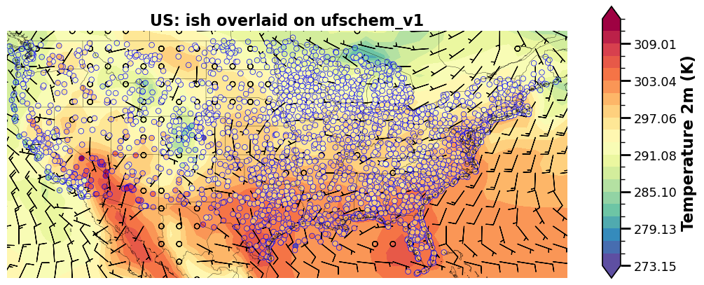
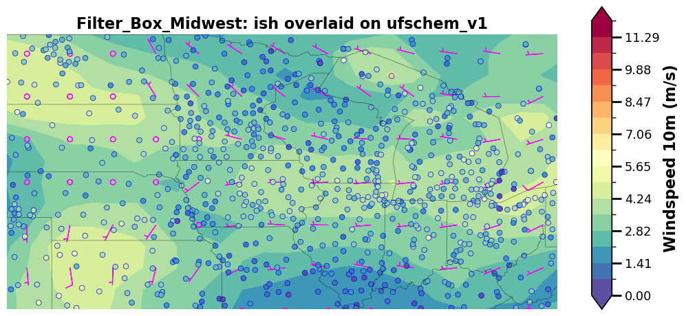
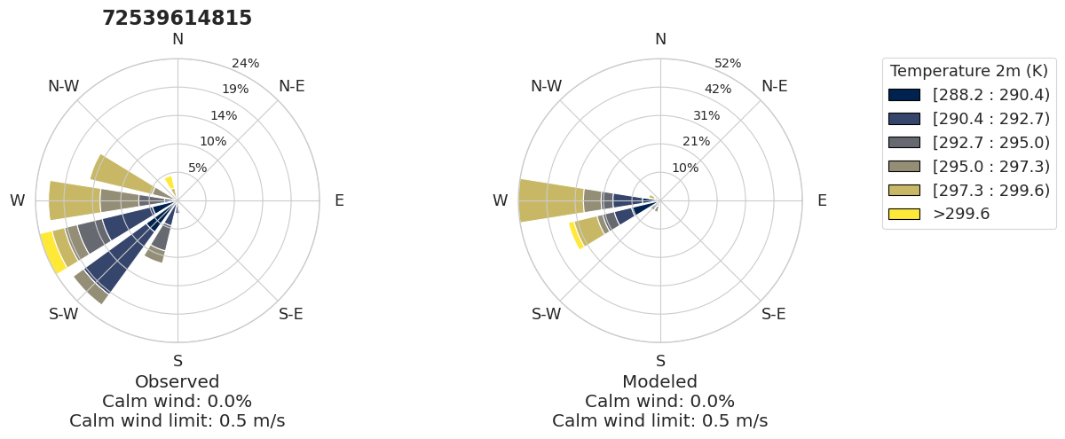
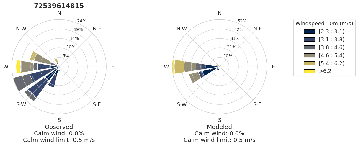
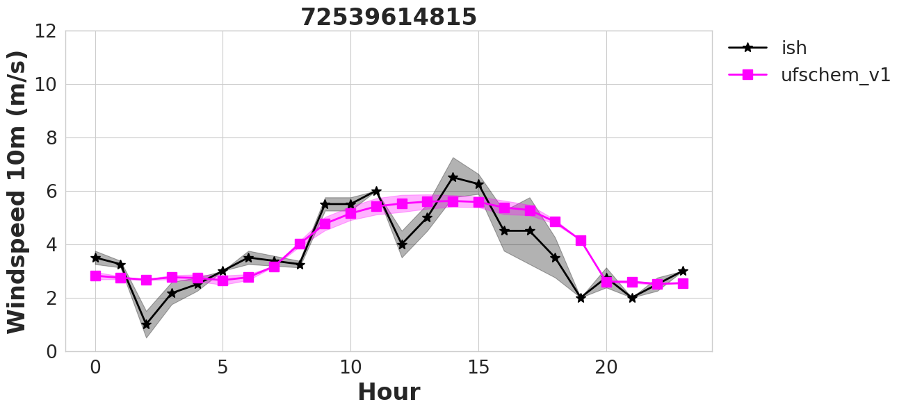
NOTE: That ISH data for calm wind sets windspeed = 0 and wind direction = 0. In the wind-rose plots, calm winds are plotted as an inner circle for wind direction and data is removed for pollution rose plots based on the threshold set in your yaml file.
All other plots, it’s up to the user on what to consider for these calm winds. Plots below and corresponding yaml file demonstrates how to remove all calm winds from the calculation for the timeseries plots (second set of plots plot_grp1a) and the spatial overlay plots (second set of plots plot_grp3a). You can see that windspeed biases go down when removing these calm winds. Additional processing and consideration for calm winds is under development.
%%time

an.plotting()
p-value annotation legend:
      ns: 5.00e-02 < p <= 1.00e+00
       *: 1.00e-02 < p <= 5.00e-02
      **: 1.00e-03 < p <= 1.00e-02
     ***: 1.00e-04 < p <= 1.00e-03
    ****: p <= 1.00e-04

ish vs. ufschem_v1: Custom statistical test, P_val:5.084e-07
p-value annotation legend:
      ns: 5.00e-02 < p <= 1.00e+00
       *: 1.00e-02 < p <= 5.00e-02
      **: 1.00e-03 < p <= 1.00e-02
     ***: 1.00e-04 < p <= 1.00e-03
    ****: p <= 1.00e-04

ish vs. ufschem_v1: Custom statistical test, P_val:0.000e+00
p-value annotation legend:
      ns: 5.00e-02 < p <= 1.00e+00
       *: 1.00e-02 < p <= 5.00e-02
      **: 1.00e-03 < p <= 1.00e-02
     ***: 1.00e-04 < p <= 1.00e-03
    ****: p <= 1.00e-04

ish vs. ufschem_v1: Custom statistical test, P_val:9.758e-92
Saving rose plot to ./output/ish_ufschem/plot_grp6.rose_plot.t.2017-07-01_00.2017-07-03_00.state.MI...


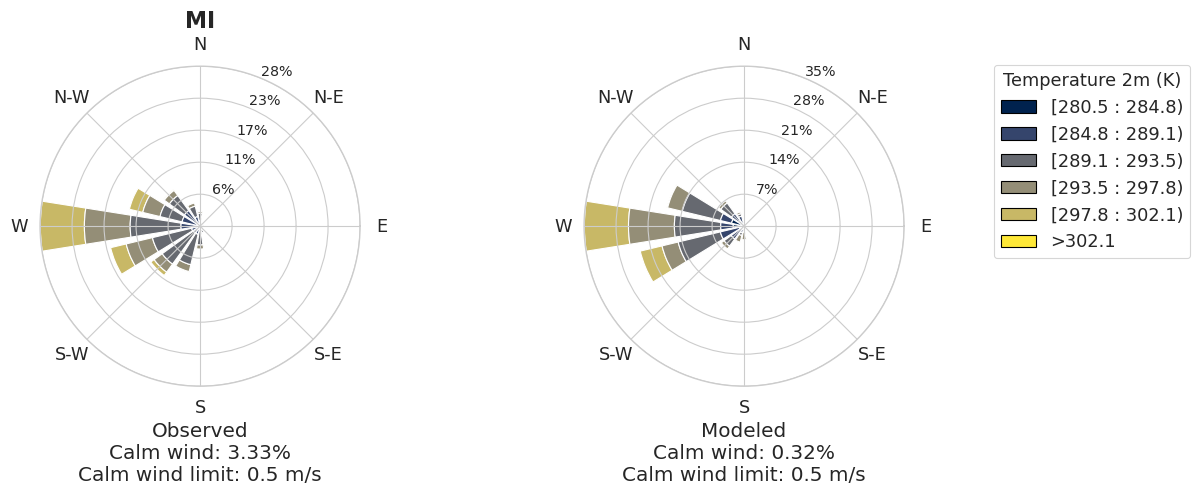
Saving rose plot to ./output/ish_ufschem/plot_grp6.rose_plot.t.2017-07-01_00.2017-07-03_00.siteid.72539614815...
Saving rose plot to ./output/ish_ufschem/plot_grp6.rose_plot.ws.2017-07-01_00.2017-07-03_00.state.MI...
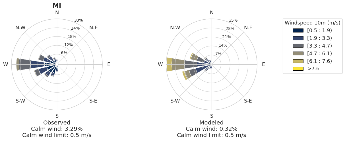
Saving rose plot to ./output/ish_ufschem/plot_grp6.rose_plot.ws.2017-07-01_00.2017-07-03_00.siteid.72539614815...
Saving rose plot to ./output/ish_ufschem/plot_grp6.rose_plot.dpt.2017-07-01_00.2017-07-03_00.state.MI...
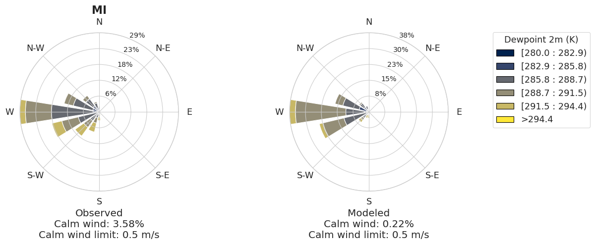
Saving rose plot to ./output/ish_ufschem/plot_grp6.rose_plot.dpt.2017-07-01_00.2017-07-03_00.siteid.72539614815...
CPU times: user 2min 29s, sys: 32.1 s, total: 3min 1s
Wall time: 2min 59s
%%time

an.stats()
CPU times: user 6.45 s, sys: 11.7 s, total: 18.2 s
Wall time: 18.3 s
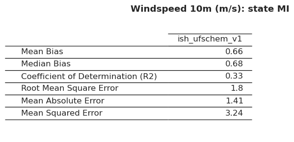
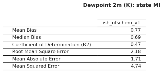
The stats routine has produced two files (one for each data variable). This is one of them:
Stat_ID,Stat_FullName,airnow_RACM_ESRL,airnow_RACM_ESRL_VCP
MB,Mean_Bias,3.93,3.23
MdnB,Median_Bias,3.86,3.27
R2,Coefficient_of_Determination_(R2),0.56,0.54
RMSE,Root_Mean_Square_Error,11.64,11.59