AirNow and CAM-chem SE (unstructured grid)

Here we show a quick example of how to compare unstructured grid model output to surface observations. Note that the sample file provided here shouldn’t be used for scientific analysis. For scientific applications, the community MUSICAv0 CONUS simulates are available at https://doi.org/10.5065/tgbj-yv18.

First we need to import the driver.

from melodies_monet import driver

Initiate the analysis class

Now lets create an instance of the melodies_monet.driver analysis class. It consists of 4 main parts: model instances, observation instances, a paired instance of both. This will allow us to move things around the plotting function for spatial and overlays and more complex plots.

an = driver.analysis()
an

analysis(
    control='control.yaml',
    control_dict=None,
    models={},
    obs={},
    paired={},
    start_time=None,
    end_time=None,
    download_maps=True,
    output_dir=None,
    debug=False,
)

Control File

Read in the required yaml control file that sets up all the definitions of what we want to pair and plot.

an.control = 'control_camchem_se.yaml'
an.read_control()
an.control_dict

Show code cell output Hide code cell output

{'analysis': {'start_time': '2019-09-05-00:00:00',
  'end_time': '2019-09-06-00:00:00',
  'output_dir': './output/airnow_camchemse',
  'download_maps': False,
  'debug': True},
 'model': {'cam-chem-se': {'files': 'example:camchem:se',
   'mod_type': 'cesm_se',
   'scrip_file': 'example:camchem:se_scrip',
   'radius_of_influence': 18000,
   'mapping': {'airnow': {'O3_SRF': 'OZONE'}},
   'projection': 'None',
   'plot_kwargs': {'color': 'dodgerblue', 'marker': '+', 'linestyle': '-.'}}},
 'obs': {'airnow': {'use_airnow': True,
   'filename': 'example:airnow:2019-09',
   'obs_type': 'pt_sfc',
   'variables': {'PM2.5': {'unit_scale': 1,
     'unit_scale_method': '*',
     'nan_value': -1.0,
     'ylabel_plot': 'PM2.5 (ug/m3)',
     'ty_scale': 2.0,
     'vmin_plot': 0.0,
     'vmax_plot': 22.0,
     'vdiff_plot': 15.0,
     'nlevels_plot': 23},
    'OZONE': {'unit_scale': 1,
     'unit_scale_method': '*',
     'nan_value': -1.0,
     'ylabel_plot': 'Ozone (ppbv)',
     'vmin_plot': 15.0,
     'vmax_plot': 55.0,
     'vdiff_plot': 20.0,
     'nlevels_plot': 21}}}},
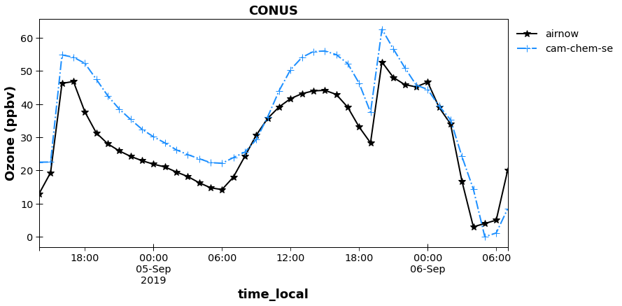
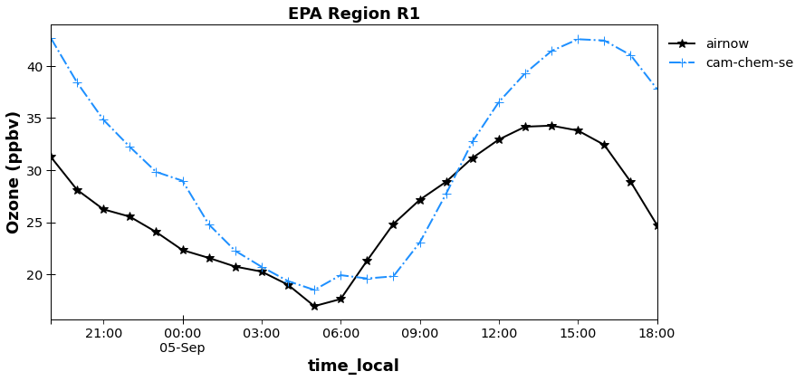
 'plots': {'plot_grp1': {'type': 'timeseries',
   'fig_kwargs': {'figsize': [12, 6]},
   'default_plot_kwargs': {'linewidth': 2.0, 'markersize': 10.0},
   'text_kwargs': {'fontsize': 18.0},
   'domain_type': ['all', 'epa_region'],
   'domain_name': ['CONUS', 'R1'],
   'data': ['airnow_cam-chem-se'],
   'data_proc': {'rem_obs_nan': True,
    'ts_select_time': 'time_local',
    'ts_avg_window': 'H',
    'set_axis': False}},
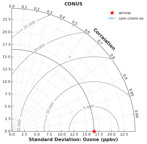
  'plot_grp2': {'type': 'taylor',
   'fig_kwargs': {'figsize': [8, 8]},
   'default_plot_kwargs': {'linewidth': 2.0, 'markersize': 10.0},
   'text_kwargs': {'fontsize': 16.0},
   'domain_type': ['all', 'epa_region'],
   'domain_name': ['CONUS', 'R1'],
   'data': ['airnow_cam-chem-se'],
   'data_proc': {'rem_obs_nan': True, 'set_axis': True}},
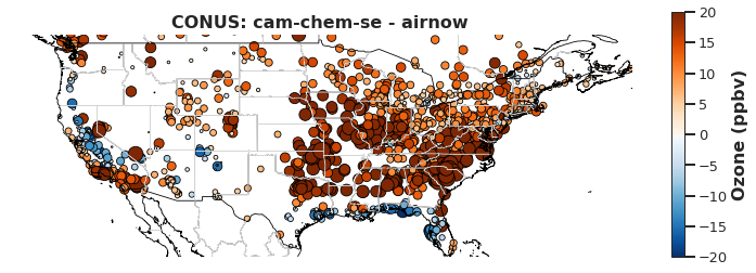
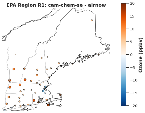
  'plot_grp3': {'type': 'spatial_bias',
   'fig_kwargs': {'states': True, 'figsize': [10, 5]},
   'text_kwargs': {'fontsize': 16.0},
   'domain_type': ['all', 'epa_region'],
   'domain_name': ['CONUS', 'R1'],
   'data': ['airnow_cam-chem-se'],
   'data_proc': {'rem_obs_nan': True, 'set_axis': True}},
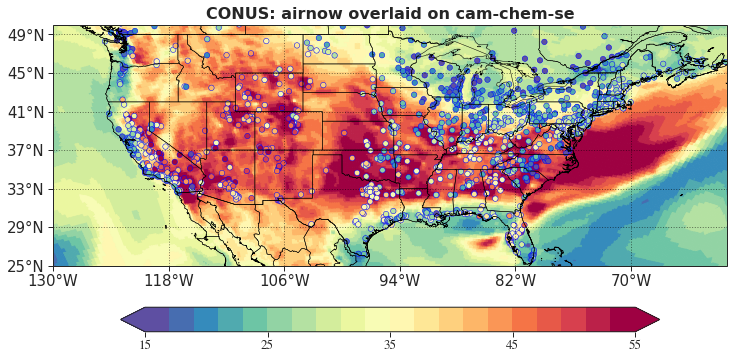
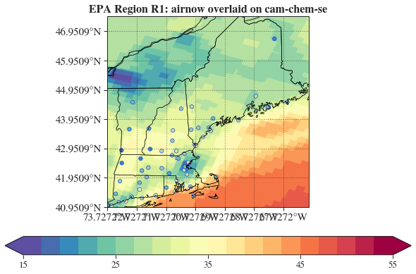
  'plot_grp4': {'type': 'spatial_overlay',
   'fig_kwargs': {'states': True, 'figsize': [10, 5]},
   'text_kwargs': {'fontsize': 16.0},
   'domain_type': ['all', 'epa_region'],
   'domain_name': ['CONUS', 'R1'],
   'data': ['airnow_cam-chem-se'],
   'data_proc': {'rem_obs_nan': True, 'set_axis': True}},
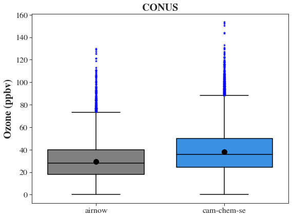
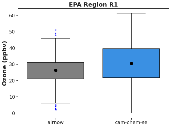
  'plot_grp5': {'type': 'boxplot',
   'fig_kwargs': {'figsize': [8, 6]},
   'text_kwargs': {'fontsize': 20.0},
   'domain_type': ['all', 'epa_region'],
   'domain_name': ['CONUS', 'R1'],
   'data': ['airnow_cam-chem-se'],
   'data_proc': {'rem_obs_nan': True, 'set_axis': False}}},
 'stats': {'stat_list': ['R2', 'MB', 'RMSE'],
  'output_table': False,
  'domain_type': ['all', 'epa_region'],
  'domain_name': ['CONUS', 'R1'],
  'data': ['airnow_cesm_se']}}

Load the model data

The driver will automatically loop through the “models” found in the model section of the control file and create model classes for each. Classes include the label, mapping information, and xarray object as well as the filenames. Note it can open multiple files easily by including wildcards. Here we are only opening one CAM-chem file.

an.open_models()

cam-chem-se
{'files': 'example:camchem:se', 'mod_type': 'cesm_se', 'scrip_file': 'example:camchem:se_scrip', 'radius_of_influence': 18000, 'mapping': {'airnow': {'O3_SRF': 'OZONE'}}, 'projection': 'None', 'plot_kwargs': {'color': 'dodgerblue', 'marker': '+', 'linestyle': '-.'}}
example:camchem:se
**** Reading CESM SE model output...

an.models

{'cam-chem-se': model(
     model='cesm_se',
     radius_of_influence=18000,
     mod_kwargs={'var_list': ['O3_SRF', 'lat', 'lon'], 'scrip_file': '/glade/u/home/cdswk/.cache/pooch/8834f0b10a87870342f40e37c461b326-ne0CONUS_ne30x8_np4_SCRIP.nc'},
     file_str='example:camchem:se',
     label='cam-chem-se',
     obj=...,
     mapping={'airnow': {'O3_SRF': 'OZONE'}},
     label='cam-chem-se',
     ...
 )}

an.models['cam-chem-se'].obj

<xarray.Dataset>
Dimensions:  (time: 24, z: 1, ncol: 174098)
Coordinates:
  * z        (z) float64 992.6
  * time     (time) datetime64[ns] 2019-09-05 ... 2019-09-05T23:00:00
Dimensions without coordinates: ncol
Data variables:
    O3_SRF   (time, z, ncol) float32 dask.array<chunksize=(24, 1, 174098), meta=np.ndarray>
    lat      (ncol) float64 dask.array<chunksize=(174098,), meta=np.ndarray>
    lon      (ncol) float64 dask.array<chunksize=(174098,), meta=np.ndarray>
Attributes: (12/13)
    ne:                         0
    np:                         4
    Conventions:                CF-1.0
    comment:                    Sample file created for MUSICA tutorial by Du...
    source:                     CAM
    case:                       f.e22.FCcotagsNudged.ne0CONUSne30x8.cesm220.2...
    ...                         ...
    initial_file:               /glade/p/acom/MUSICA/restart/ne0CONUSne30x8/f...
    topography_file:            /glade/p/cesmdata/cseg/inputdata/atm/cam/topo...
    model_doi_url:              https://doi.org/10.5065/D67H1H0V
    time_period_freq:           hour_1
    mio_has_unstructured_grid:  True
    mio_scrip_file:             /glade/u/home/cdswk/.cache/pooch/8834f0b10a87...

# All the info in the model class can be called here.
print(an.models['cam-chem-se'].label)
print(an.models['cam-chem-se'].mapping)

cam-chem-se
{'airnow': {'O3_SRF': 'OZONE'}}

# All the info in the analysis class can also be called.
print(an.start_time)
print(an.end_time)
print(an.download_maps)

2019-09-05 00:00:00
2019-09-06 00:00:00
True

Generate plots

%%time

an.plotting()

AirNow and CAM-chem SE (unstructured grid)

Initiate the analysis class

Control File

Load the model data

Open Obs

Pair model and obs data

Generate plots